Ana Sayfa
Hakkimizda
Ürünler
İletişim
Ürün Bulucu
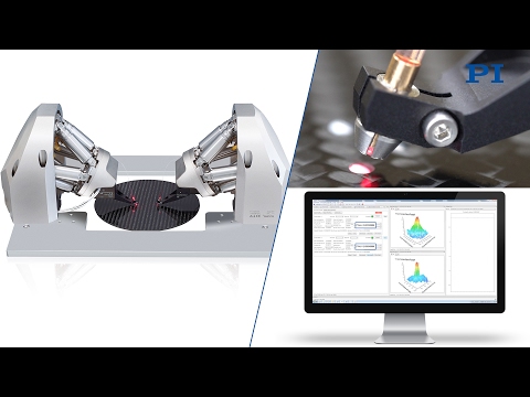
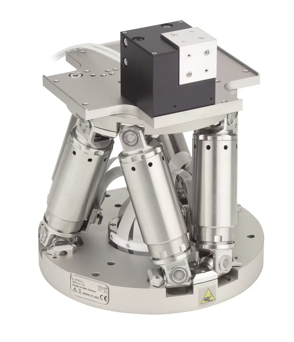
PI - Nanopositioning Piezo Flexure Stages PI - Miniature Stages PI - Linear Stages PI - Linear Actuators PI - Rotation StagesPI - XY StagesPI - HexapodsPI - Engineered Subsystems for AutomationPI - Fast Multi-Channel Photonics AlignmentPI - Software SuitePI - Controllers & Drivers PI - Piezoelectric Transducers & Actuators PI - Air Bearings & StagesPI - Sensors, Components & AccessoriesPI - Vacuum